Linear Regression Still Going Strong

October 4, 2024

A brief history of linear regression

Linear regression was performed long before the advent of computers. The least squares method, which is now the foundation of linear regression, was published by Adrien-Marie Legendre in 1806 in the appendix of his books on the paths of comets. Carl Friedrich Gauss claimed that he had been using the method of least squares as early as 1794, notably for calculating the orbit of Ceres.

Various specialists using linear regression

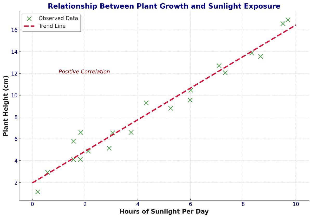
The linear least squares (LLS) approximation for linear function isn’t only for predicting planetary movements. Biologist can use it to study the relationship between the amount of sunlight a plant receives and its growth. Psychologist might use it to predict anxiety based on the amount of social media usage. Sociologist may employ it to explore whether there is a gender gap in lawyers incomes. In epidemiology, regression models provided early evidence linking tobacco smoking to increased mortality and morbidity through observational studies.

What model can tell us

Linear regression is used across many fields and industries, answering various types of questions:

• One is a hypothesis testing, to see if there is an association between two variables. For instance, in studying whether gender impacts income, we are interested in whether salary (Y) changes based on a binary variable representing gender (X).
• Second is a strength of association, it helps describe how closely two variables are related, typically measured by the correlation coefficient $r$, ranging from -1 to 1, or $r^2$, which ranges from 0 to 1. For example, if the $r^2$ between hours of sunlight per day and plant height after 3 months is 0.81, it means that knowing the amount of sunlight allows you to predict plant height fairly accurately. On the other hand, if $r^2$ for the relationship between tobacco smoking and lifespan is 0.19, knowing whether someone smokes would not provide enough information to predict their lifespan with high accuracy.
• The final answer is determining the equation of the best-fitting line, expressed as $Y = a + bX$, where $Y$ is the predicted value for a given $X$, $a$ is the $Y$ intercept (the value of $Y$ when X is zero), and $b$ is the slope (the change in $Y$ for each unit increase in $X$). For example, the equation $Anxiety\, Level = a + b*(Social\, Media\, Use)$ can be used to model the relationship between social media usage and anxiety.

Why is linear regression so popular

Linear regression remains one of the most fundamental concepts in statistics and data analysis for several reasons.

• The equation of the straight line is simple and easy to understand, making linear regression a good candidate for exploratory analysis because of great explainability

• Although linear regression assumes a straight-line relationship, which may not always fit the data, many extensions and variation (e.g. polynomial regression) have been developed to handle more complex relationships.

• For simple linear regression, only two variables (independent and dependent) and relatively few data points are needed to build the model, making it highly accessible

Conclusion

While modern data science has given us more advanced models like GPT-based chatbots or diffusion-based text-to-image models, linear regression continues to be foundational. Even when you are asking a tool like ChatGPT to create a trend line, it often leverages linear regression under the hood to provide you insights.

View this page on GitHub.